Semantic Image Segmentation Software
Project overview
A small team’s task: build and compare two contrasting approaches to image segmentation, a classical pixel-based method and a machine-learning model, then extend one of them with depth-camera data, evaluating both against the SUN RGB-D and NYU Depth v2 benchmark datasets using IoU, Dice score, and pixel accuracy. My own contribution was the classical segmentation pipeline and the performance-metric calculations used to evaluate every method in the report, a teammate developed the machine-learning model (a ResNet-U-Net, later extended with depth fusion). This satisfied the brief’s requirement for two genuinely different segmentation paradigms, not two variants of the same approach. The project is complete.
System architecture
The classical pipeline converts each image into the perceptually uniform CIELAB colour space, smooths it with a mean-shift filter to suppress false edges while preserving real boundaries, enhances local contrast with adaptive histogram equalisation to bring out weak edges in dark regions, then runs Canny edge detection with thresholds set dynamically from each image’s own gradient statistics rather than a single fixed threshold, since the right threshold varies a lot between scenes. A final pass of morphological closing, dilation, and region-filling turns the resulting edge map into clean, enclosed regions.
Selected engineering challenges and decisions
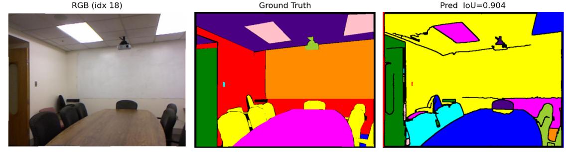
Not trusting a single quantitative metric over what the result actually looks like. Across both datasets the classical method scored a pixel accuracy of around 69 to 70% and an average IoU of roughly 0.65 to 0.68, fast and competitive without any training data. Looking at individual scenes rather than just the averages surfaced something the headline numbers hid: the worst-scoring result by IoU actually had visibly better segmentation than the best-scoring one, because the ground truth labels themselves were coarse for that scene, merging detailed structure into one large region.
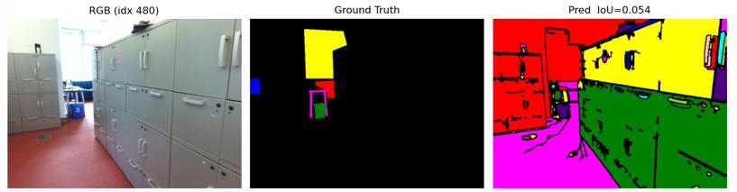
The reverse was also true: a clean, well-labelled ground truth elsewhere misleadingly inflated the score for an image where the edge detector had actually missed real boundaries. This mattered because a metric is only as trustworthy as the ground truth it’s measured against, treating IoU as ground truth itself would have meant drawing the wrong conclusion about which result was actually better.
Current status
Completed: the classical pipeline, the evaluation metrics, and the cross-dataset comparison are all finished and reported. This was a closed university assessment; no further development is planned.
What I learned or am proud of
The most useful outcome wasn’t the accuracy numbers, it was the reminder that a single quantitative metric can disagree with what your eyes tell you, and that’s worth checking before trusting the number. I now treat that as a standing check on any evaluation I run: look at the actual outliers, not just the aggregate score, because the aggregate can be telling you about the measurement, not the result.