Solar Inverter Reverse Engineering Project
Project overview
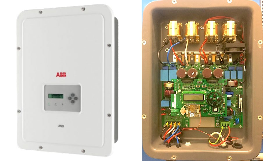
A small team’s task: reverse engineer a commercial single-phase grid-connected solar inverter (a 5kW ABB UNO string inverter), then analytically model and simulate its two power conversion stages to predict efficiency, losses, and thermal performance at real operating points. This is an analytical study, not a build, the deliverable is a validated model of an existing commercial product, not new hardware. The project is complete and closed.
System architecture
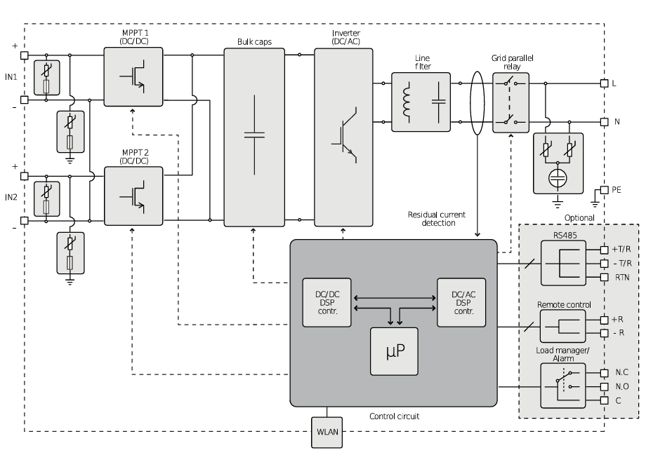
The manufacturer’s own datasheet gave a first, general picture of the architecture before any teardown: two MPPT DC-DC stages feeding shared bulk capacitors into a DC-AC inverter stage, with a DSP-based control system and grid-interface protection (a residual current monitor, a grid-parallel relay) around it.
Opening the physical unit confirmed the actual topology: a DC-DC boost stage handling maximum power point tracking, followed by a full-bridge DC-AC inverter stage producing grid-compatible AC output.
Selected engineering challenges and decisions
Explaining efficiency behaviour, not just stating a number. A single efficiency percentage doesn’t say why a converter behaves the way it does across its operating range, so I categorised every loss mechanism in the boost stage by how it scales with current: constant losses (gate drive, off-state leakage, diode reverse-recovery switching), losses linear in current (diode conduction, MOSFET switching), and quadratic losses (inductor and MOSFET conduction, capacitor ESR, all I²R-type losses). This mattered because it turns “the converter is 99% efficient” into an explanation of why: at low current, the small constant losses dominate and efficiency is climbing; past a peak, the quadratic I²R terms take over and efficiency falls away again, a real performance trade-off, not a fixed number.
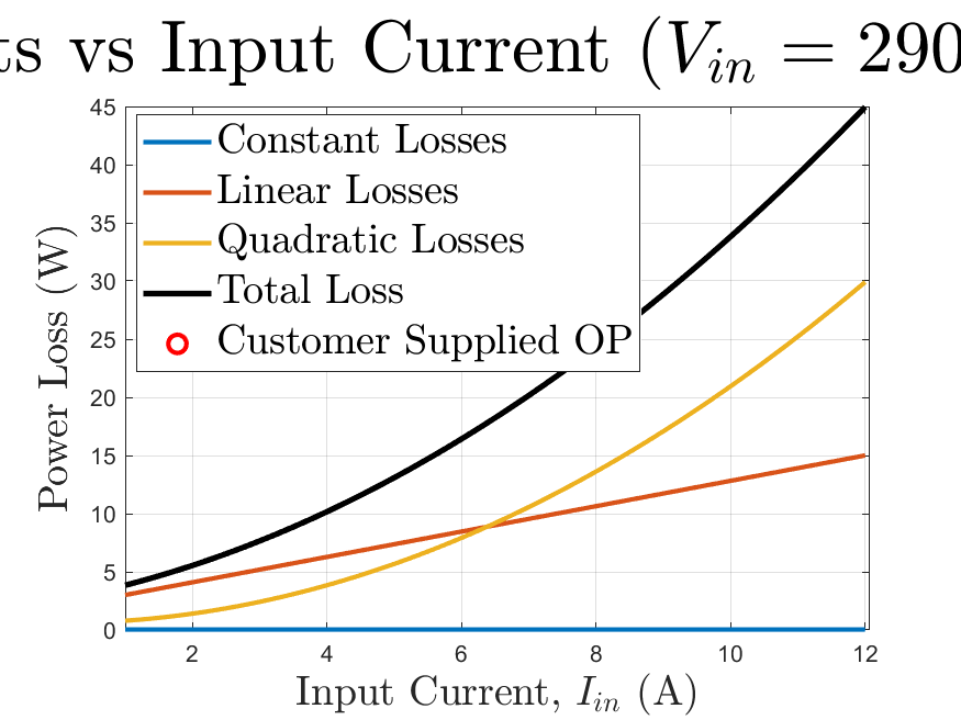
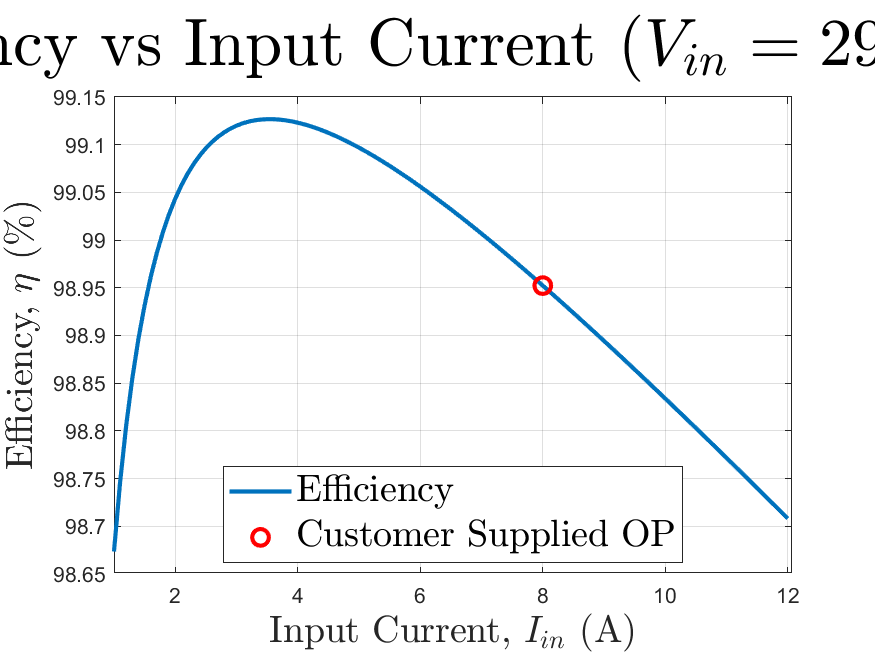
At the customer-specified operating point (8A input, 290V in, 400V out), the breakdown is concrete: roughly 1.9W constant, 8.8W linear (diode conduction dominant), and 13.6W quadratic (inductor conduction dominant), for about 24.3W of total loss against 2320W input power. The efficiency curve below shows what that breakdown implies: it peaks around 3.5A and falls on both sides, and the customer’s 8A point sits past the peak, on the side where the quadratic terms are starting to dominate.
Verification or evidence
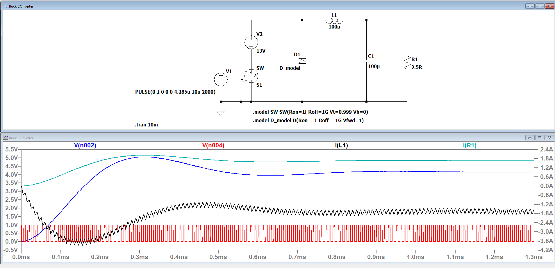
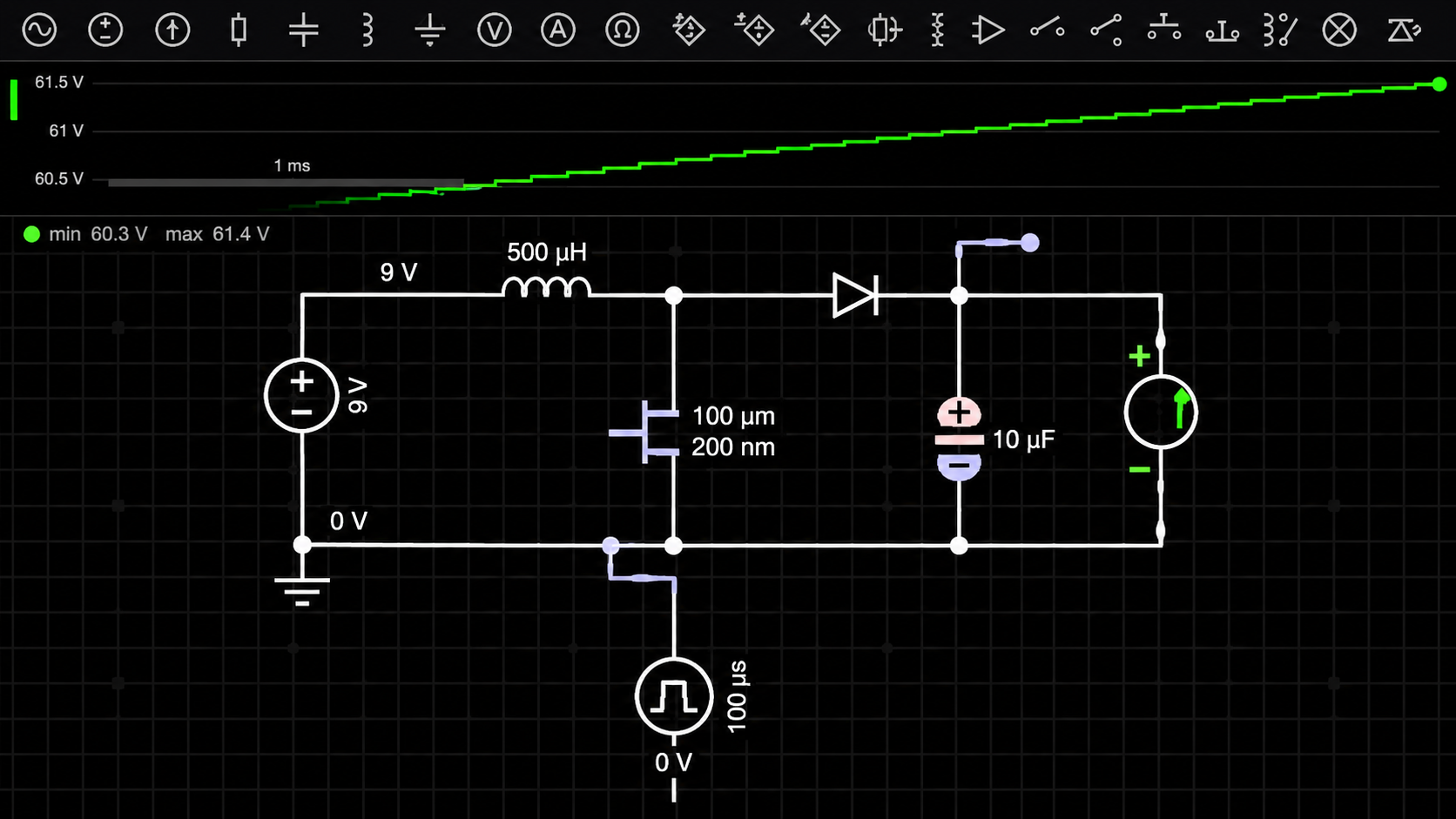
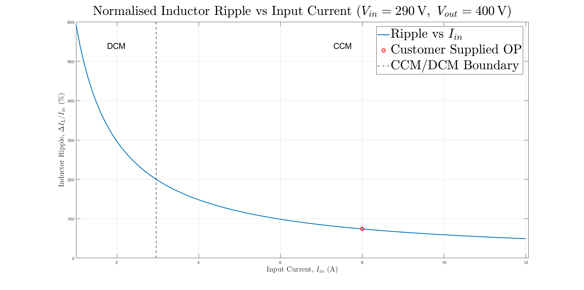
Component values and ratings, derived from datasheets and physical inspection, were checked through hand calculations and both idealised and realistic LTspice simulations (the realistic models included real component parasitics). The boost converter’s inductor ripple was checked across its full input current range to confirm continuous-conduction-mode operation at the specified point, not the discontinuous mode the analysis assumes:
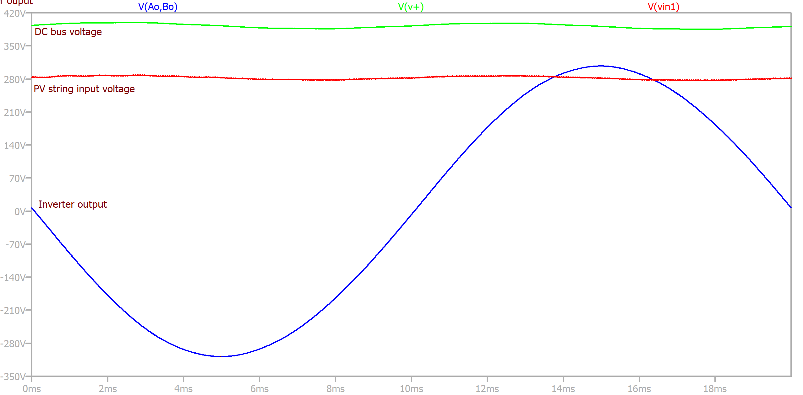
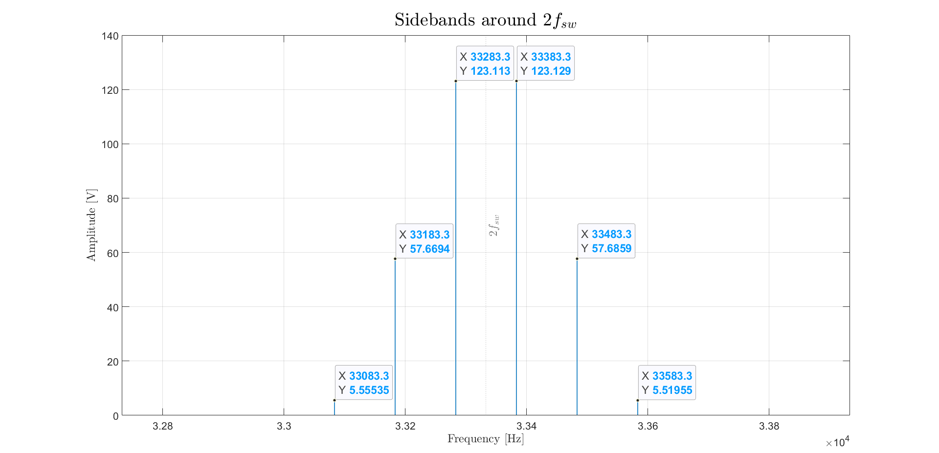
The two stages were also combined into one full-system simulation, to check the whole power path worked end to end rather than just each stage in isolation, and the full-bridge stage’s switching harmonics were checked against where the analysis predicted them:
A thermal model also confirmed every component stayed within its safe operating temperature even at full rated load.
Current status
Completed: the analytical and simulated results agreed closely at both operating points, giving simulated efficiencies of around 98 to 98.6%, in line with the inverter’s published peak efficiency of 97.4%. This was a closed university assessment; no further development is planned.
What I learned or am proud of
Categorising losses by how they scale with current, rather than stopping at a single efficiency figure, is what actually explains the converter’s behaviour: it shows where the efficiency peak comes from, and why a real operating point chosen for other reasons (the customer’s specified 8A) doesn’t land on it. That’s the transferable habit I’d take into any efficiency analysis, decompose a result into the mechanisms that produce it before treating the headline number as the answer.
Gallery